Contents
- Preface
- Introduction
- Literature and Economic Theory
- Research Method
- Findings and Discussion
- Conclusions
- Bibliography
- Appendix I
- Appendix II
- Appendix III
Preface
This is a copy of my disseration research project, with names redacted. It was written in 2022/23. While it uses some OpenAI libraries, it’s not using generative artificially intelligent economic agents (like LLMs).
Introduction
Artificial Intelligence (AI) has traditionally been confined to science fiction, however, following advances in computer science; mathematics; and processing power, the economy has rapidly pivoted and adopted AI, with corporate investment in AI increasing thirteenfold from $14bn in 2013 to $189bn in 2022, with 2021 seeing a record $276bn (Maslej, et al., 2023).
Though research into AI’s economic impact is emerging, a dearth of empirical evidence remains at the intersection of the disciplines. This poses an acute problem for policymakers, particularly in competition policy, where decisions made today could stifle technological progress, or encourage inegalitarian transfer of wealth to the capital holding classes.
We’re pressing all the gas pedals at once on this one. Heading towards a utopia, or a dystopia… Some kind of ‘topia’ for sure. But we’re getting there real fast (Murphy, 2023)
Profit seeking firms are increasingly adopting AI to automate pricing strategies (The Economist, 2022). AIs, tasked with price-optimisation, use heuristics to spot patterns and relationships between multiple items, giving firms an insight into competitor ability-to-supply, and consumer willingness-to-pay, which are non-obvious to human price setters.
{Redacted}, an AI-price-optimisation supplier, is quoted suggesting AIs do not lead inexorably to higher prices, however the existence of services which distribute the same AI-generated price list to many discrete clients may lead to passive collusion for firms operating in similar markets, and could lead to prices inflated above competitive Nash equilibria. They may additionally create societal deadweight losses - where output is lower than the economy would maximally allow - resulting in sub-optimal welfare & utility attainment. Alternatively, they may resolve extant deadweight losses, though do so by assigning excess utility to firms, rather than consumers.
This research focuses on empirically testing outcomes in a simulated economy, where firms in a homogeneous market subscribe to the same AI price-optimisation supplier and adopt their pricing strategies. The research is conducted by:
- Creating a small economy simulator in python.
- Training AI-Agents using reinforcement-learning to interact with the economy under each of the canonical market structures (Monopoly, Duopoly, Oligopoly, and Perfect Competition).
- Testing if the AIs behave according to expectations in each market structure, or if they demonstrate cooperative behaviour, collusive behaviour, or cause inegalitarian utility outcomes.
Competition theory expects that market structures with low numbers of firms to induce higher prices, while higher numbers of firms competitively induce low prices near to firms’ marginal costs. The results of this project’s research into AI competition did not fully align with these expectations. Across all structures AIs demonstrated behaviour that closely resembled passive collusion among firms, consistently choosing a cooperative price point, rather than an expected competitive price point. Consumers persistently faced prices above the wholesaler rate. Relatively lower prices were observed in some perfectly competitive structures as anticipated, though these prices were still higher than marginal costs.
In addition to demonstrating collaboration in pricing, AIs cooperated in unpredicted ways. When running the simulator under the assumptions of Bertrand competition (firms are price-setting, not quantity-setting), AI-firms autonomously identified that they could use the price input as a proxy for quantity-setting. 7/10 vendors consistently identified the consumers’ maximal aggregate willing-to-pay value, then wilfully set their prices above the maxima, extricating themselves from the market. The remaining 3/10 organised into an oligopoly, cooperating to increase prices, and creating a deadweight loss. In this model, AI-firms demonstrated behaviour as if they existed under the Cournot quantity-setting competition rules, even though they were programmed under Bertrand’s model.
Literature and Economic Theory
Historical Context
Economists have long considered the impact of machines on society, and the winners & losers they create. In his work, The Principles of Political Economy and Taxation, Ricardo questions the influence of machinery on the interests of the different classes of society (Ricardo, 1817). Over the course of the coming decades, forced by the emergence of Artificial Intelligence, humanity will contend with similar existential questions relating to egalitarianism; distributional justice; labour; and capital, in the face of disruptive technology.
Bertrand & Cournot Models of Competition
Bertrand’s model and its counterpart, Cournot’s model, are the underlying systems of competition in the research’s simulation. The way AI interact in these models forms the bulk of the research Findings section.
The Bertrand model works under the assumption that firms set a price-point at which they are willing to supply products, for example soda, to the market. Thereafter, consumers purchase as many cans of soda as demanded (Varian, 2014, p. 530). The model doesn’t allow for quantity as an input, and firms have unlimited capacity to supply soda to the market.
The model posits that, excluding monopolies, market power isn’t a significant factor, as firms will behave under the assumption of perfect competition - forced through Bertrand’s Paradox to supply at a price point at or near the marginal cost of production. Firms attempting to raise prices above marginal costs will lose their consumers to firms supplying nearer to marginal costs. The model doesn’t account for quantity as an input, and assumes the firm has an unlimited capacity to supply soda to the market.
Cournot’s model approaches competition under the assumption that firms set quantity-points, and the market price is then set by consumption patterns (Cournot, 1838). For markets with a low number of firms (high concentration), a dominant firm’s choice to increase output reduces market-wide price (due to the laws of supply and demand, where high supply induces low prices). In markets where there are low numbers of firms, those price reductions land proportionately on each firm in the market. In a market with two soda firms, the quantity-adjusting firm attracts 1/2 of the losses incurred by their own supply increase. When acting as profit-maximising rational agents, firms in markets with high concentrations do not increase their supply above loss-making quantity-points (except if a temporary increase may force a weaker firm out of the market).
Deadweight Loss
In the Cournot Model, with the option to quantity-set, firms have a mechanism to under-supply the market, creating a deadweight loss. This loss is a cost to society, shared between firms and consumers respectively, in the form of a suboptimal profitability and welfare attainment. This market inefficiency is illustrated in Figure 2.1, the monopolist, able to choose their quantity-supplied, elects to produce at QF, before their marginal costs (MC) begin to increase beyond profits. The firm, acting entirely rationally by avoiding loss-making sales, create an allocatively inefficient deadweight loss to society.
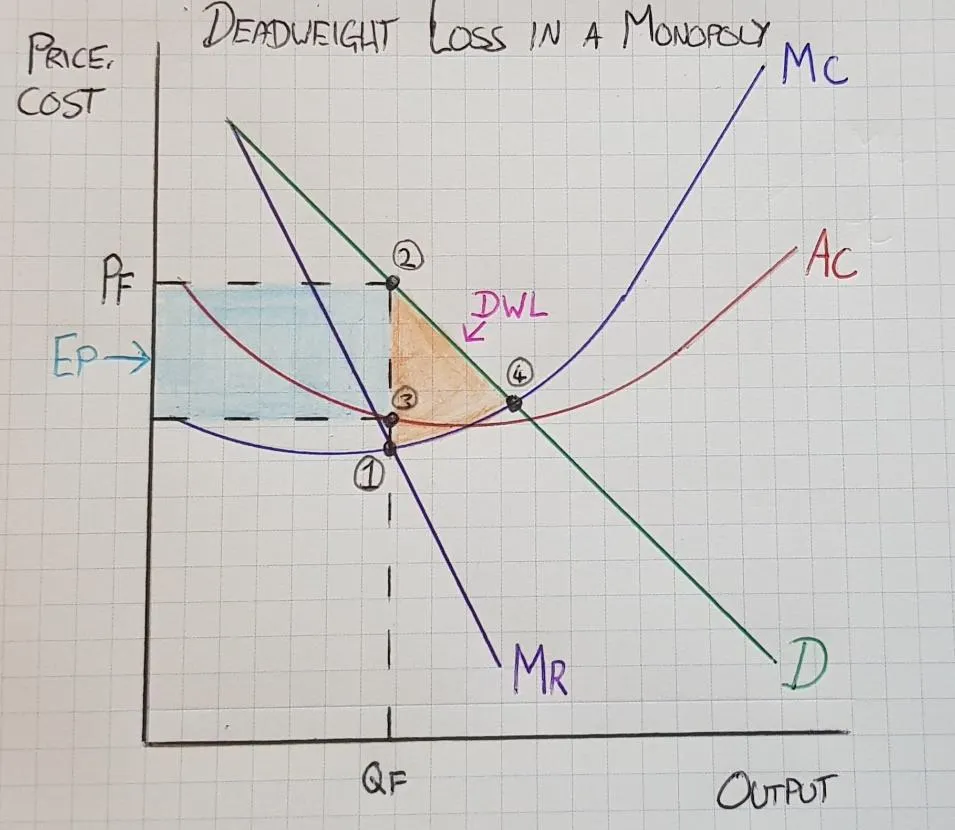
- Figure 2.1 - Societal losses under monopoly conditions
Market authority overseers aim to avoid these deadweight losses where possible. Concerned that their regulatory framework may not sufficiently protect consumers, a 2018 Financial Conduct Authority discussion paper proposed that firms are responsible for making sure that all their customers are treated fairly (FCA, 2018).
This market inefficiency can be resolved in one of two ways. Through competition where more firms enter the market to supply the deficit of soda, resolving the consumer-side loss of welfare. Alternatively, firms with sufficient market power can apply price discrimination tactics, charging the actual price consumers are willing-to-pay shifting Figure 2.1’s Marginal Revenue (MR) curve alongside its demand (D) curve.
Under normal circumstances, finding the willingness-to-pay of all consumers (in order to supply along the MR curve) would incur significant search costs for the firm. However, with the assistance of AI-price-setting algorithms, these search costs may no longer be burdensome.
Both scenarios resolve the market inefficiency from an allocative point of view (there are no consumers with money to spend on consumption left wanting), however they have different societal outcomes. Competition equitably distributes the deadweight loss between firms and consumers, while price discrimination distributes the deadweight loss entirely to firms. Passive cooperation between AI-firms creates a risk of these societally suboptimal outcomes being achieved, while leaving consumers unaware of their welfare loss.
These inegalitarian allocations of utility (a form of wealth transfer), favours firms over consumers, and may fall foul of the duty of care expected from the FCA between firms and their consumers. This transfer of utility through allocatively-efficient resolution is a core reason that the interplay of supply and demand in no way rules out the possibility of large and lasting divergence in the distribution of wealth (Piketty, 2014), a once extant relationship which Piketty argues prompted Marx and Engels to publish Das Kapital and The Communist Manifesto.
Reinforcement-Learning, AI, and Economics
Using reinforcement-learning, AI are trained through iterative competitive episodes, analogous to games in Game Theory. AIs understand the rules of the game and their own objective but are not explicitly programmed with strategy. AIs compete against copies of themselves millions of times, slightly adjusting strategy in each iteration commensurate with outcomes of all previous games. Unsuccessful strategies which don’t increase its reward are discarded, while successful strategies are adopted. Over millions of iterations, the AI builds its optimal reward-maximising strategy, equivalent to a utility-maximisation strategy.
The reinforcement-learning technique used to train AI in this research is OpenAI’s Gym framework (Brockman, et al., 2016), applying the Proximal Policy Optimization (PPO) algorithm (Schulman, et al., 2017). The algorithm is illustrated in Figure 2.2. AIs recursively suggest an Action to take, and a prediction of its Reward (for example, Action: increase price by $1 | Expected Reward: +$0.50 profit). The simulation is then run with that Action applied. In response, the AI receives a reward, and an Observation containing the new state of the simulation. If the reward exceeds expectations, the iteration’s Action is adopted into the Agent’s Policy going forward, and will be used to inform future actions, and unsuccessful Actions are discarded. In each discrete market structure, AI all progress through these steps in unison, competing for optimal utility. This iterative procession gradually converges on an optimal policy for each AI during training.
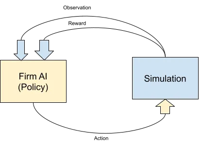
- Figure 2.2 - Recursive simulation loop, after (Sutton & Barto, 2018, p. 86)
This iterative adoption of strongest policies (Dynamic Learning) is analogous to the Schumpterian approach to Dynamic Economic change, where creative destruction brings about better outcomes over time (Schumpeter, 1942). The analysis in Section 4 will incorporate an evolutionary approach, as suggested in An Evolutionary Theory of Economic Change (Nelson & Winter, 1990), where changes in state are observed over time (Simonetti, 2010), as well as focusing on converged equilibrium states, per neoclassical approaches.
One-shot and iterative games
Reinforcement-learning’s evolutionary pattern has consequences for the way AI should be modelled in game theory. Figure 2.3 illustrates output decisions for a Duopoly in a one-shot prisoner’s dilemma. For both firms, the best strategy when considering the other firm’s strategy, is to supply a High Output to the market, reducing profits. This Nash equilibrium, where two equilibrium points lead to the same expectations for the players (Nash, 1950, p. 2), of [Defect:100 + Defect:100 = 200] incentivises firms to supply at egalitarian societally optimal low prices. For firms, this is a sub-optimal outcome, a higher aggregate output is available in the system at [Cooperate:200 + Cooperate:200 = 400].
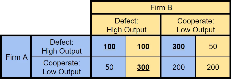
- Figure 2.3 - Prisoner’s dilemma, after (Harding & Harding, 2019, p. 56)
Across many games (which AIs necessarily take part in during iterative training), there is the opportunity to trial cooperative strategies in a non-punitive environment before the AIs face real-world scenarios. Through this evolutionary process, AI-Firms learn to trust, ultimately developing high-trust cooperative strategies, undermining egalitarian high-supply-low-price points.
Game Theory in Machine Learning (CEPR)
A working paper from CEPR (Centre for Economic Policy Research) describes the creation of a small economy simulator, and unexpected behaviour of AI-agents in a Cournot Oligopoly structure (Pastorello, et al., 2019).
Agents, without an opportunity to explicitly collude, were found to passively collude to increase prices, to the detriment of the economy’s consumers. Figure 2.4 shows the cooperation persisting, even after manual intervention by researchers forces Agents to the Nash price, whereafter Agents return to their pre-intervention collusive price point. CEPR’s AIs demonstrated a textbook high-trust tit-for-tat strategy (Dixit & Nalebuff, 1991). Note that, although the AI pushed prices above the Nash Price, they don’t push prices all the way towards the cooperation price, rather adopting a price point between the two.
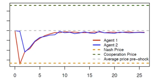
- Figure 2.4 - cooperative AI pricing found in CEPR’s research
Research Method
To test if AI Agents demonstrate collusive behaviour in each market structure, the researcher created a small economy simulator in Python, then trained 36 AI Agents in the following canonical market structures.
| Competition models available | Market structure | Number of AI-Firms | Number of consumers | Training iterations |
|---|---|---|---|---|
| Bertrand, Cournot | Monopoly |
1 |
25 |
2,000,000 |
| Bertrand, Cournot | Duopoly | 2 | 25 | 3,000,000 |
| Bertrand, Cournot | Oligopoly | 5 | 25 | 5,000,000 |
| Bertrand, Cournot | Perfect Competition | 10 | 25 | 15,000,000 |
Simulated Competition Models
The simulator’s competition model code supports two variations, Bertrand and Cournot. In Bertrand, all AI-Firms simultaneously set prices, then consumers are invited to purchase. In Cournot, all AI-Firms simultaneously set both quantity and prices, then consumers are invited to purchase until the AI-Firms are no longer willing to supply. In both models, there is no product differentiation and consumers face no search costs.
Simulated Consumption Patterns
AI-Firms in the simulation face consumers with finite money, but infinite desire. Consumers in the economy are utility-maximising, and the only source of utility is consumption of the product. The simulator initialises with $19 distributed to each of 25 consumers, totalling $475 for the entire economy per episode.
Within their budget, consumers can purchase any quantity, so long as AI-Firms are still supplying. Consumers do not accrue or carry forward funds between episodes. In Bertrand, because AI-Firms are willing-to-supply an unlimited volume at their price point, all consumers purchase at the same lowest offered price. In the Cournot Model, consumers can purchase at different prices, so long as there are still vendors willing-to-supply. For example, the following are valid consumption configurations:
Bertrand
- 3 products at $6 each, leaving $1
- 1 product at $12 each, leaving $7
- 19 products at $1 each, leaving $0
Cournot
- 1 product for $12 each, leaving $7
- 19 products at $1 each, leaving $0
- 3 products at $6 each and 1 product at $1, leaving $0
Consumer’s money remaining at an episode’s end is their individual Deadweight Loss, and the aggregate of these remainders is the economy-wide deadweight loss.
Simulated Supply Patterns
AI-Firms have access to an unlimited wholesaler, supplying the product at a flat $8 rate. In addition to the flat rate, AI-Firms have a V-shaped marginal cost curve (Figure 3.1), initially starting at $5 per transaction, descending by $0.66 per transaction for six transactions to simulate economies of scale, after which the marginal cost increases continuously by $0.66 per transaction to simulate diseconomies of scale. Marginal cost schedules are discrete per AI-Firm, and not shared across the economy, or across episodes.
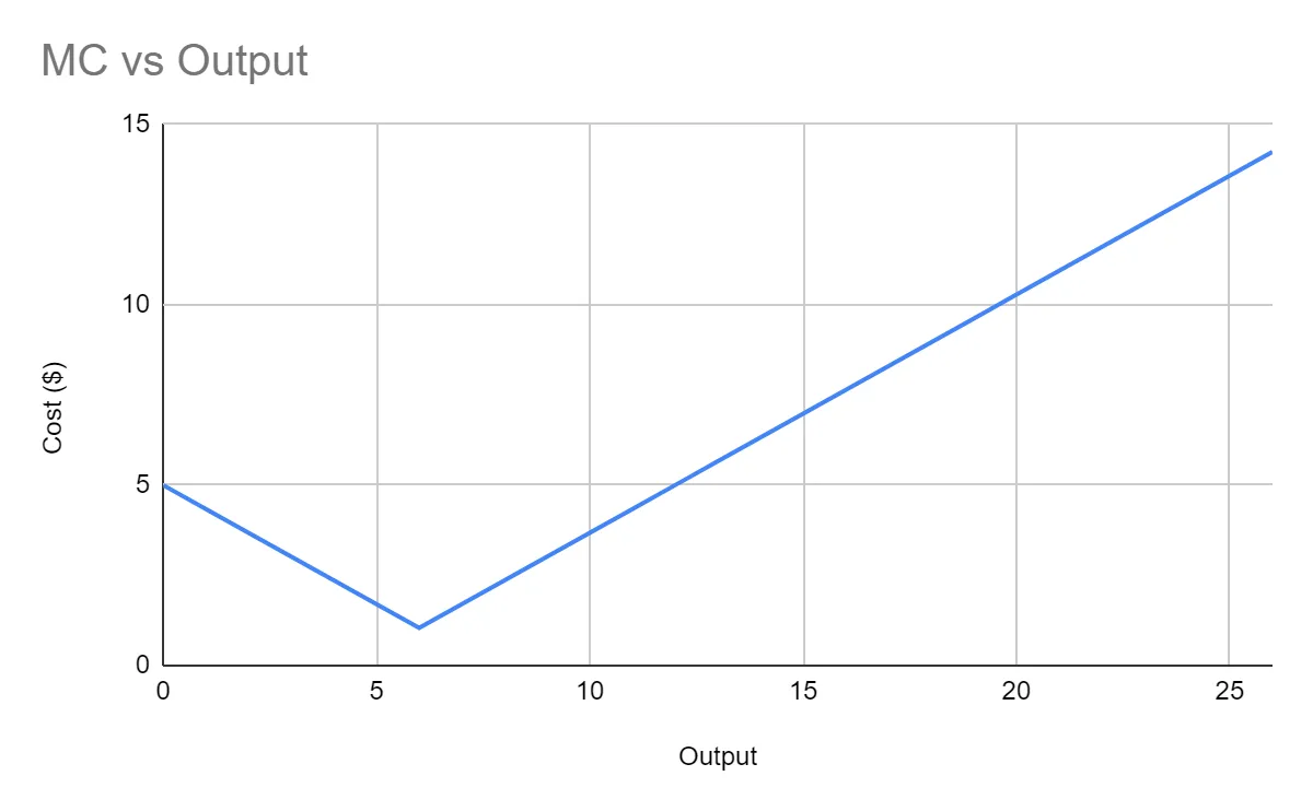
- Figure 3.1 - AI-Firms’ MC
AI-Firms’ price points are decided at the beginning of each episode simultaneously. Points begin at $8 and increase in whole integers of $1 to $38. A table of profit/loss points is available in Appendix I. In Cournot, AI-Firms additionally set quantity points - which begin at 0, and increase in whole integers up to 30.
A technical description of the simulator from a software engineering perspective can be found in Appendix II.
Limitations
There are limitations to this approach. Training AIs via reinforcement-learning is computationally and temporally expensive. Both factors increase with complexity of the model. The research is conducted on a consumer-grade laptop, where the simulation takes up to 60 hours, creating some restrictions on experimentation.
These computational restrictions mean that some variables have been modelled with less fidelity than ideal, for example, prices available to AI-Firms are whole integers (eg. 1, 2, 3, 4), even though the competitive and cooperative optimal may sit at a fractional figure, this can create an unnatural single price equilibria if the industry is large enough (Dixon, 1993). Some variables have been held ceteris paribus, even though results would be richer with a mutatis mutandis approach, for example a consumer willingness-to-buy through a diminishing marginal utility function has not been modelled. Some variables are smaller than ideal, the model for perfect competition has only ten AI-Firms, and the entire economy is modelled with only 25 consumers sharing $475. Appendix II contains an additional technical implementation limitation. In the Cournot model, AI-Firms can freely enter and exit the market by setting their quantity-point to 0, which closely simulates Perfect Competition, however in Bertrand, AI-Firms don’t have this option by default.
To produce focused results, the models follow narrow neoclassical assumptions. Obeying the three neoclassical ‘prongs’ as described in The Econocracy (Earle, et al., 2017, p. 38), where rational agents are individualistic, in that they work to their own benefit above all else; optimising, in that relentlessly work to improve their reward; and equilibrium-seeking, in that they work until no actor in the economy has incentive to deviate. This narrow approach falls foul of The Lucas Critique which (although originally raised in a macroeconomic context) argues (Lucas, 1976) that simple models which consist of optimising agents are not necessarily appropriate for generalised quantitative evaluation.
Finally, the models don’t consider potential human price-setters. In a perfectly competitive market, an additional non-AI price setting firm could freely join the market, marginally undercut AI-Firms’ cooperative price-point, and attract 100% of the market demand. The Human-Firm could even subscribe to {redacted}s price-optimisation service, gain access to the pricing schedule generated by AI, and marginally undercut those prices, again attracting 100% of the economy’s consumers.
Structure of results for analysis
While undergoing training the simulator records statistics about the economy using Tensorflow (Abadi, et al., 2015). Graphs are produced in TensorBoard, and will be used to show the research findings. Tabulated summary findings will also be made available in Appendix III.
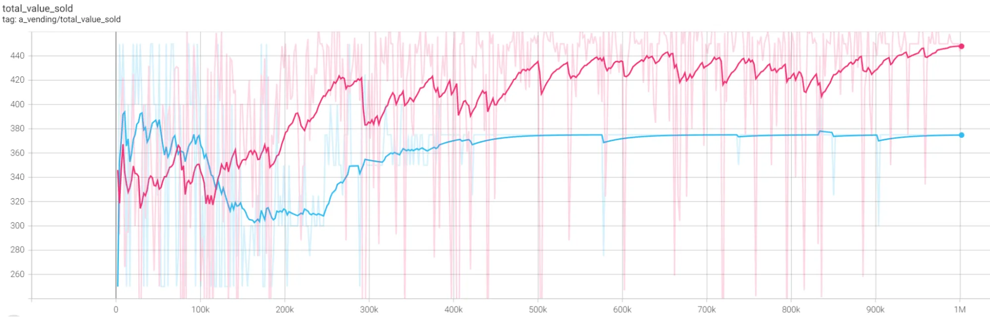
As an example, Figure 3.2 shows the learning trends of two AI training sessions across 1 million episodes in the Cournot model. The episode number is represented in the horizontal axis, while the Total Sales $Value is represented in the vertical axis. The coloured lines represent the AI-Firms’ economic output (Monopoly in orange, Duopoly’s pair in pink).
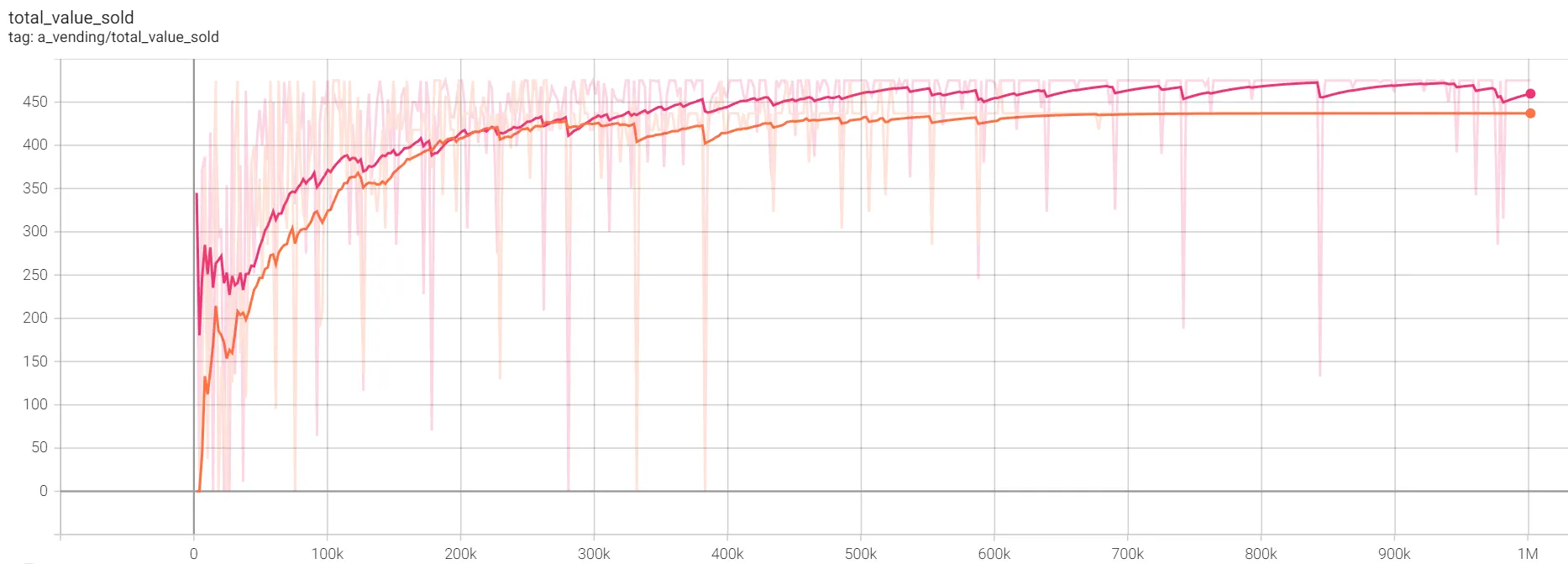
- Figure 3.2
Initially, the orange monopolist can be seen attempting to supply the market at low price-points of $200 in the early stages, before learning it can charge at a price point of $19, finally settling at $437 (a deadweight loss of $38) near the 600k episode. The pink duopolists follow a similar strategy trend, but learn they can extract the full $475 from consumers. The right-hand-side of the graph represents the strategy the AI has converged on, and would adopt in real-world pricing scenarios.
Overview of Available Statistics
| Variable | Description |
|---|---|
| Average accepted price point | Averaged value of all completed sales |
| Average offered price point | Averaged value of all prices offered, even if a sale is not successful |
| Average final vending cost | Averaged marginal cost of the final unit sold by each firm, ignoring vendors which didn't complete any sales |
| Average quantity offered | Average of all vendor quantities offered to the market |
| Count of vendors which did make a sale | Number of firms which successfully sold at least 1 unit |
| Count of vendors which did not make a sale | Number of firms which did not successfully sell at least 1 unit |
| Total Sales | The sum of all sale made, represents the number of individual units sold |
| Total Sales $Value | The sum of the $-value of all sales made, the inverse of which is the deadweight loss |
These statistics reveal the behavioural patterns of the AI-Firms during their training regime and offer insight into how they interact with each other and with the economy's consumers.Findings and Discussion
The research findings are outlined with commentary below, broken down by market structure, comparing how firms behave in Bertrand and Cournot models.
Quantitative Monopoly Results
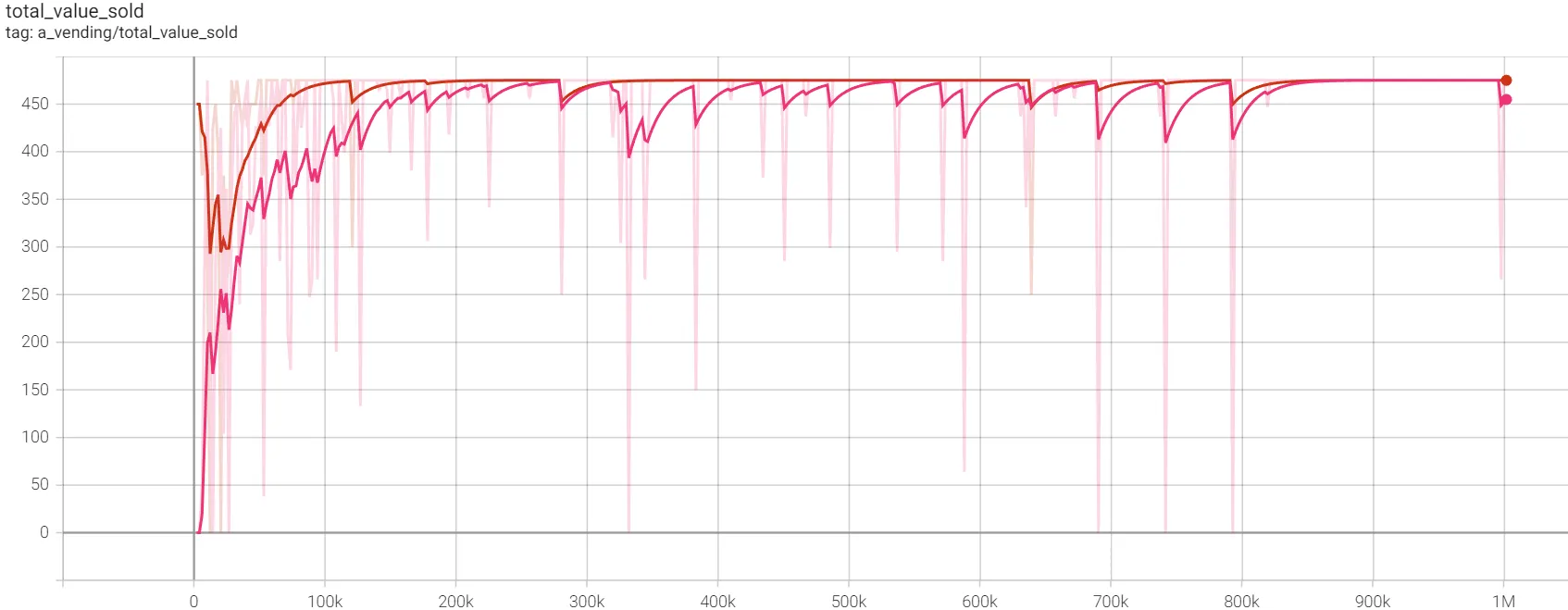
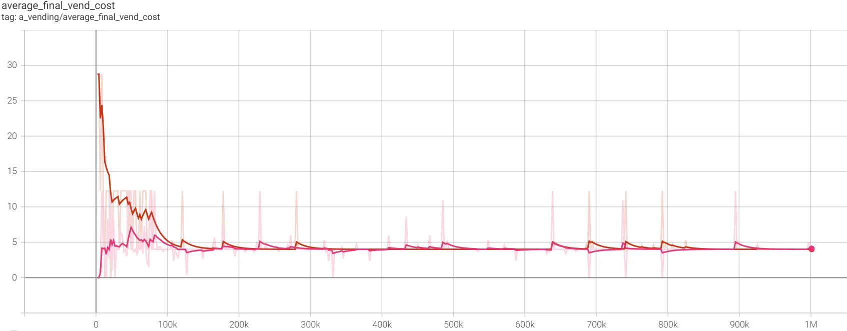
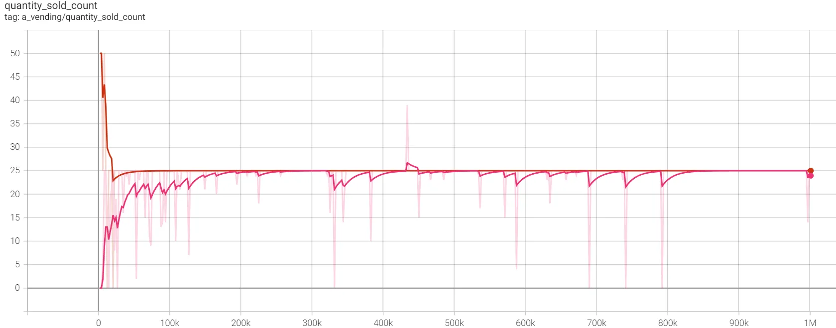
Data in Appendix III Table 1 show the results of training sessions in the Monopolist market structure after 1M iterations. The AI reached a stable equilibrium strategy at 700k iterations for both models. The results show the quantity-setting monopolist avoiding loss-making sales, and creating a deadweight loss of $38, as shown in Figures 4.1 and 4.2.
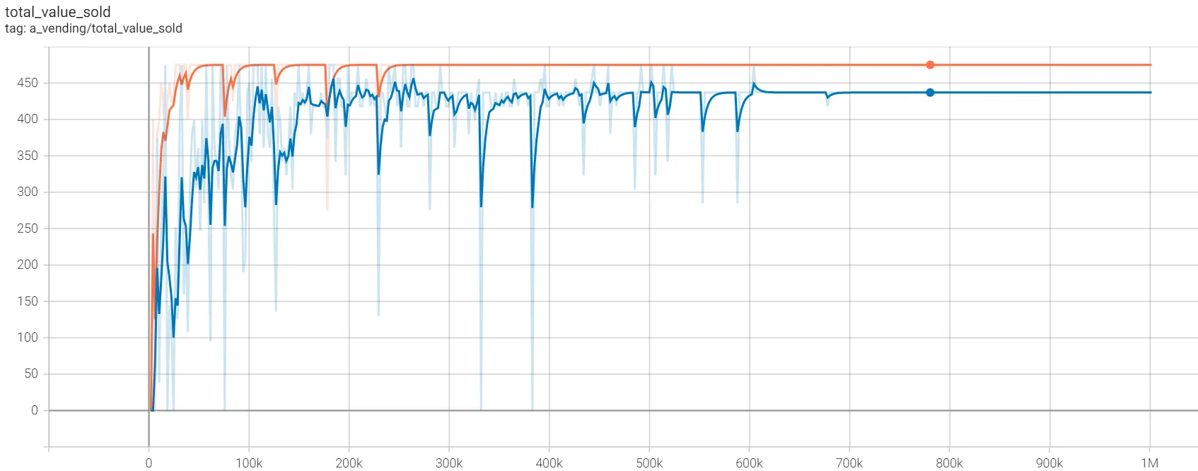
- Figure 4.1 (above) - trend for Total Sales $Value. Cournot monopolist in blue, Bertrand in orange.
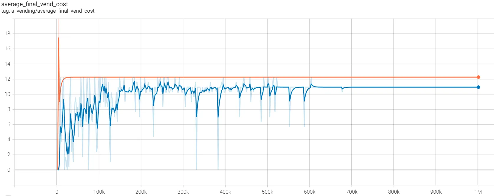
- Figure 4.2 (above) - trend for Average Final Vending Cost (Marginal Cost). Cournot monopolist in blue, Bertrand in orange.
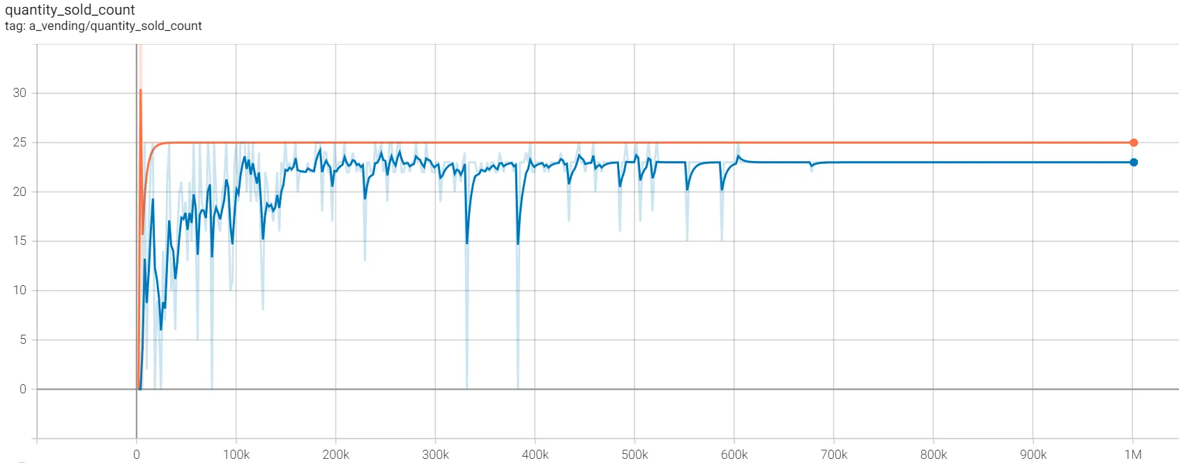
- Figure 4.3 (above) - trend for Total Quantity Sold. Cournot monopolist in blue, Bertrand in orange.
The table in Appendix I shows the 24th and 25th items sold at $19 incur losses of $0.60 and $1.26 respectively. The Cournot monopolist, with its quantity-setting mechanism, avoided selling the final two loss-making items, even though there was market demand for them, creating a deadweight loss as illustrated in Section 2 Figure 2.1. The Bertrand monopolist, without access to a quantity-setting control, subsumed the totality of the consumer budget of $475, creating no deadweight-loss. It did however suffer higher marginal costs as a result.
Quantitative Duopoly Results
Data in Appendix III Table 2 show the results of training sessions in the Duopolistic market structure, with up to two vendors, after 3M iterations. The AI reached a stable equilibrium strategy at 1M iterations for both models.
- Figure 4.4 (above) - trend for Total Sales $Value. Cournot duopolies in pink, Bertrand in orange.
- Figure 4.5 (above) - trend for Average Final Vending Cost (Marginal Cost). Cournot duopolies in pink, Bertrand in orange.
- Figure 4.6 (above) - trend for Total Quantity Sold. Cournot duopolies in pink, Bertrand in orange.
- Figure 4.7 (above) - number of vendors making sales. Cournot duopolies in pink, Bertrand in orange.
In both training sessions, duopolies can be seen voluntarily exiting the market to check if the monopolist structure returns higher aggregate profit. In the Cournot model, firms opt out by setting their quantity supplied to 0. In the Bertrand model, firms do not have direct access to this mechanism, but identify that they can set their price as a proxy above the consumer budget of $19 to exit the market.
- Figure 4.8 (above) - trend for Average Final Vending Cost (Marginal Cost) for Cournot monopolists in blue, versus Cournot duopolists in pink. When working together, the duopolists avoid the penalties incurred in diseconomies of scale, face considerably lower marginal costs, and extract more of the consumer’s budget than the monopolists, and so remain a duopolistic pair to maximise profits.
The optimal cooperative price/supply point for the Duopolies is $19 with a supply of 25, evenly sharing the quantity supplied, taking it in turns to supply product 13. The duopolies achieve this price/quantity combination in both models. Had competitive pressures been a concern for the Cournot duopolists, any price point in the range $11 - $18 could have profitably supplied more than 25 units to the market. The duopolists create inegalitarian outcomes.
Quantitative Oligopoly Results
Data in Appendix III Table 3 show the results of training sessions in the Oligopoly market, with up to five vendors, after 5M iterations. In the Bertrand model, the AI reached a stable equilibrium strategy at 1M iterations, and the strategy persisted unchanged for 300k iterations. The Cournot model failed to reach a stable equilibrium in some dimensions.
- Figure 4.9 (above) - trend for Total Sales $Value. Cournot oligopolists in orange, Bertrand in green.
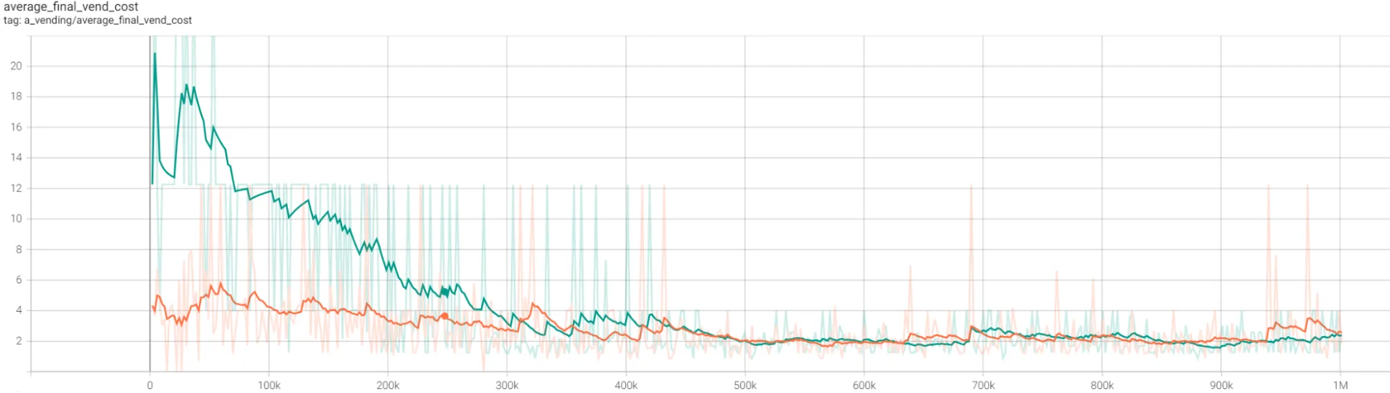
- Figure 4.10 (above) - trend for Average Final Vending Cost (Marginal Cost). Cournot oligopolists in orange, Bertrand in green.
Bertrand oligopolists established an equilibrium supplying at $18, while Cournot supplied at $19. This is peculiar. As described in the duopolist results, the price-setting Bertrand firms have the capacity to behave as quantity-setters-by-proxy & arrange as the more profitable Cournot oligopoly if they chose to.
The Bertrand oligopolists failed to recognise that they could arrange into the more efficient structure, causing deadweight loss of $25, and facing a sub-optimal marginal cost of $2.03, instead of $1.82. This result is similar in nature to the CEPR paper, where a cooperative price was established, but not the optimal cooperative price.
- Figure 4.11 (above) - trend for Total Quantity Sold. Cournot oligopolists in orange, Bertrand in green.
With additional firms, oligopolists reduce their shared exposure to diseconomies of scale, and face much lower aggregate marginal costs than the duopolies or monopolies. In both models, agents learn to cooperatively under-supply the market at a point of 25 units, creating inegalitarian outcomes.
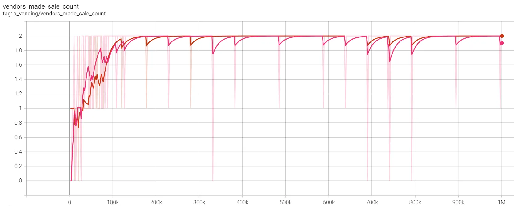
- Figure 4.12 (above) - trend for the number of vendors successfully making at least one sale during the first million training iterations. Cournot oligopolists in orange, Bertrand in green.
The AIs face considerable challenges establishing an equilibrium in this market structure, however in most episodes, at least one firm chooses to extricate itself from the market, sacrificing itself to drive aggregate profits up.
- Figure 4.13 (above) - trend for the number of vendors successfully making at least one sale between 2M - 3M iterations. Cournot oligopolists now in blue, Bertrand in red.
Bertrand settled into an equilibrium of 3 firms, while the Cournot oligopolists continued to face challenges converging on a structure. Cournot firms even begin re-testing a 5-firm structure, but learn shortly after 2.7M iterations that there are higher profits to be made between the 3-firm and 4-firm structures.
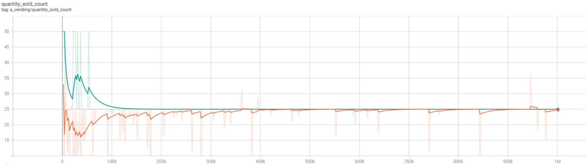
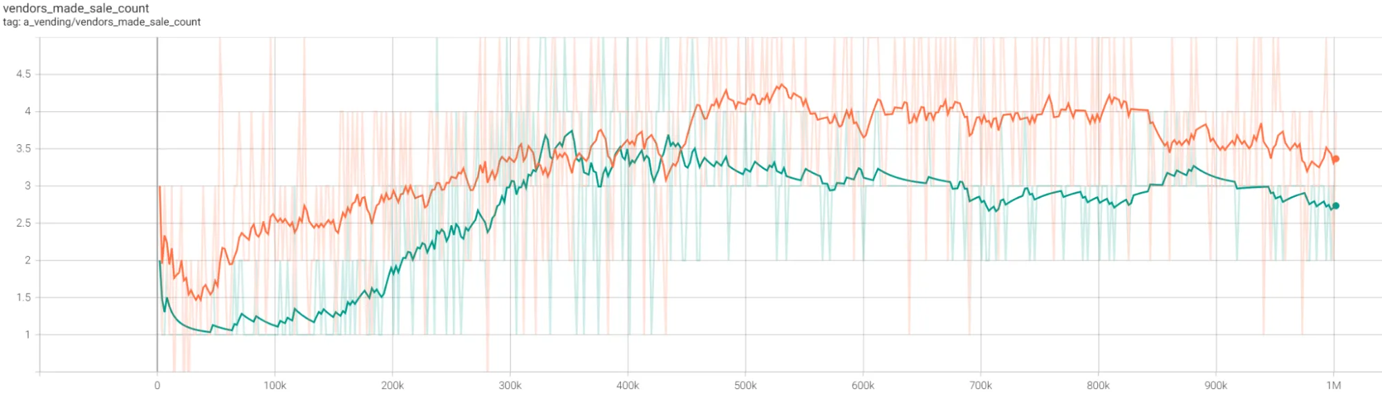
Quantitative Perfect Competition Results
Data in Appendix III Table 4 show the results of training sessions in the Perfect Competition, with up to ten firms, after 15M iterations. In Bertrand, AIs reached a converged strategy for prices at 1M iterations. Both struggled to fully converge in other dimensions, trialling adjustments even as they approached the 15-millionth iteration.
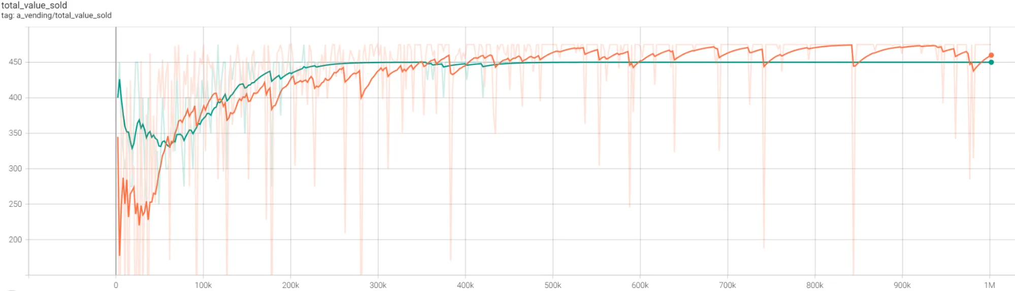
- Figure 4.14 (above) - trend for Total Sales $Value for the first million iterations. Cournot vendors in pink, Bertrand in blue.
Bertrand quickly establishes a total quantity sold at $375, a strategy causing $100 deadweight loss, from which it never deviates. Meanwhile Cournot establishes at $475, subsuming the entirety of the consumer budget.
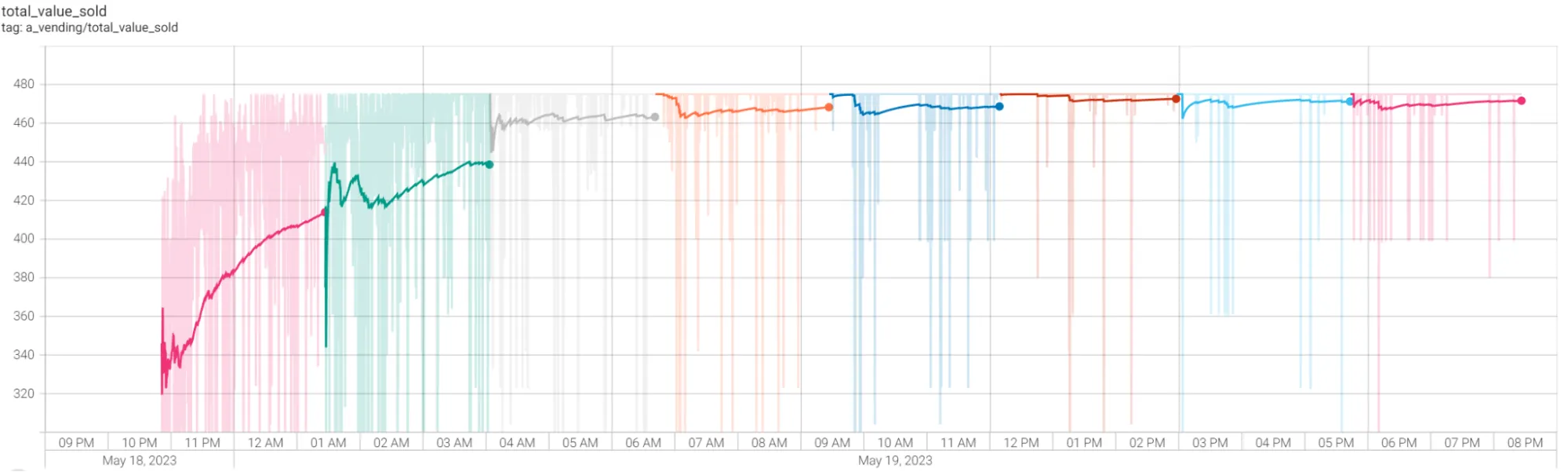
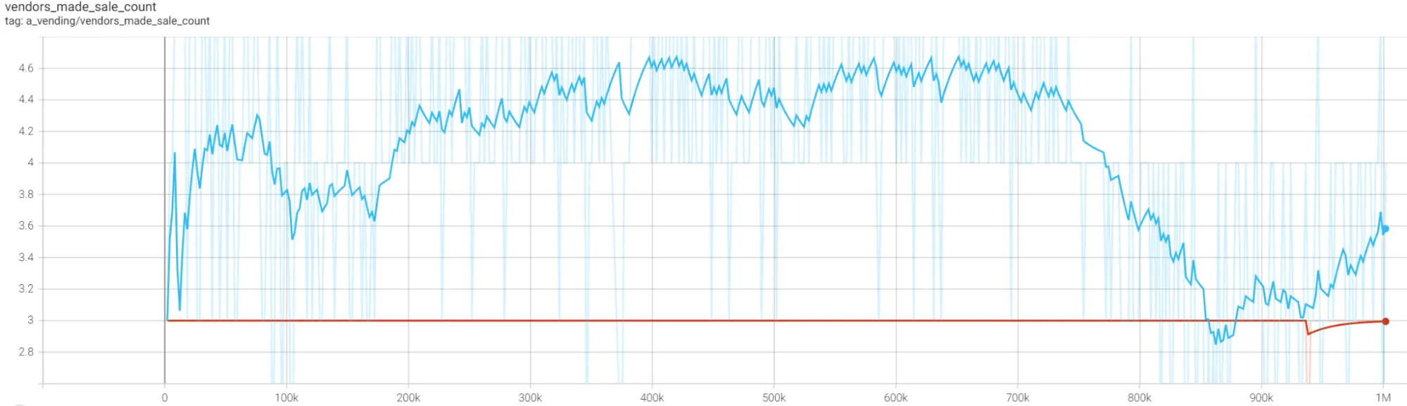
- Figure 4.16 (above) - trend for Total Sales $Value for vendors in the Cournot model across 8M iterations (colour changes denote n-millionth iteration, while the horizontal axis now represents the iteration, denoted by the time of day the simulation was running). Cournot firms consistently trial new price points, but have reliably converged at the full $475 by the 8-millionth iteration.
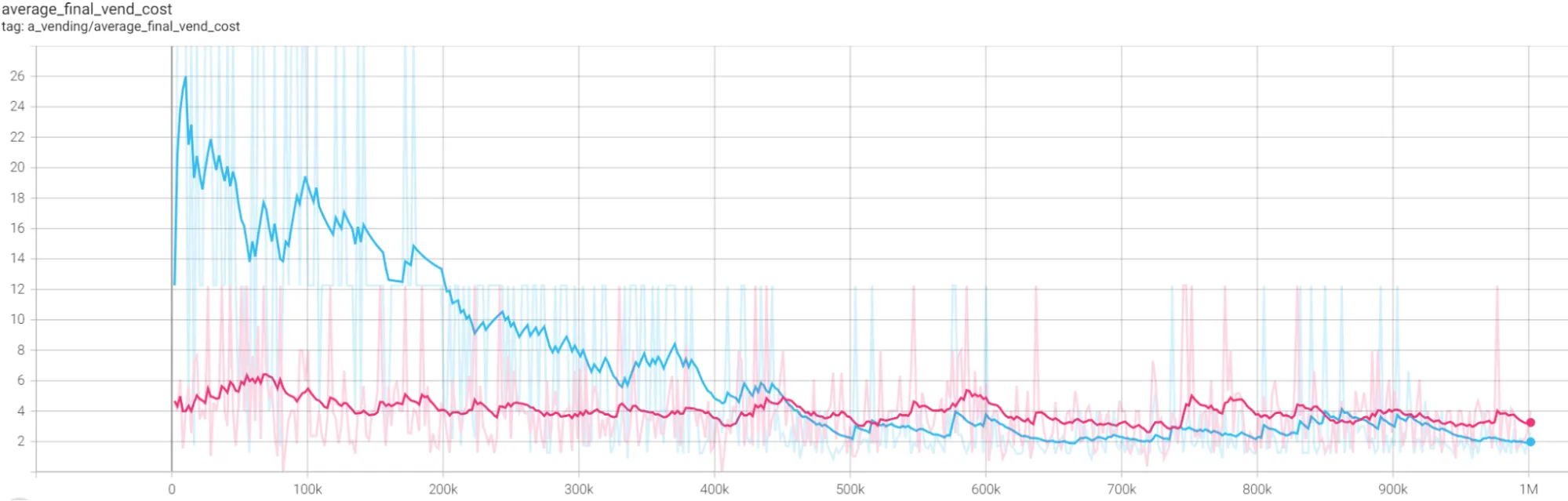
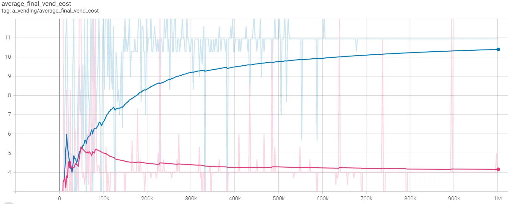
- Figure 4.17 (above) - trend for Average Final Vending Cost (Marginal Cost). Cournot vendors in pink, Bertrand in blue.
The falling Marginal Cost in Figure 4.17 is explained by the increasing vendor count in Figure 4.18. As additional vendors enter the market. Proportionally, each one shares less of the burden of diseconomies of scale. In the Cournot model, the vendor count stabilises at 2, while in Bertrand, the vendor count stabilises at 3. Note that the simulation is configured with up to 10 vendors in this mode, and more than half of the AIs opt to extricate themselves from the market.
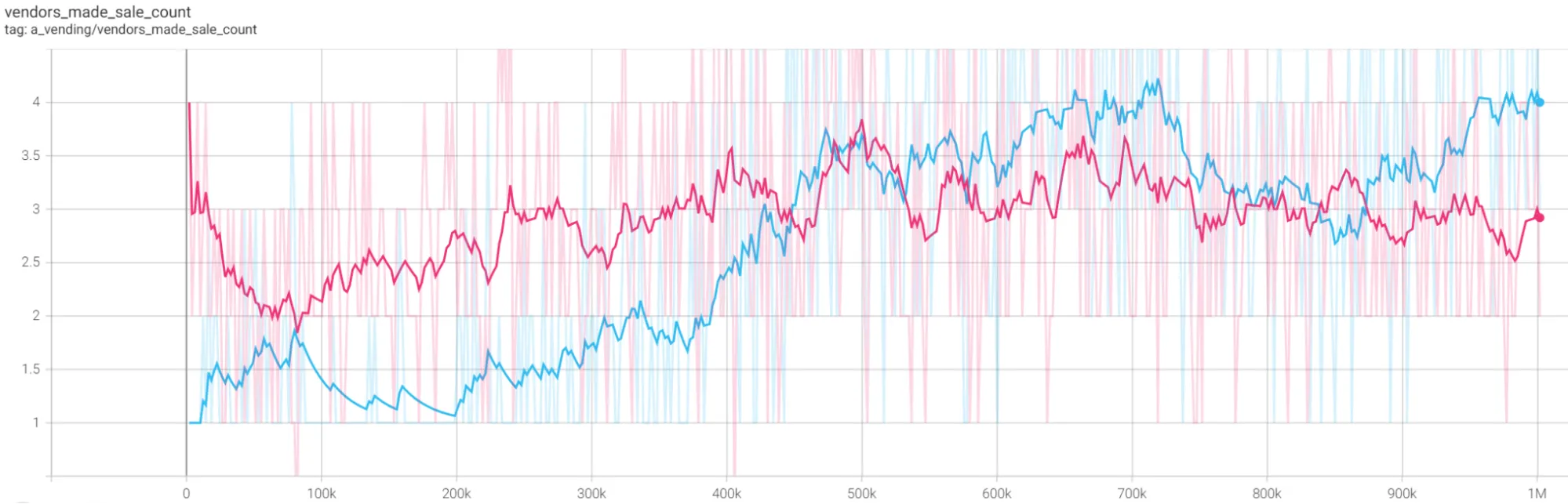
- Figure 4.18 (above) - trend for the number of vendors successfully making at least one sale during the first million training iterations. Cournot vendors in pink and Bertrand blue.
Bertrand vendors achieved the highest deadweight loss of any cohort at $100, but did so by charging the lowest price at $15 per unit. This price isn’t reflective of a full Nash equilibrium, but is considerably lower than the $18-19 price point in the other cohorts, and is supportive of evidence in CEPR’s paper, where a price point between the Nash price and cooperation price was established. Strangely, the low price point was achieved by only three of ten vendors suggesting that the risk of competition from the self-excluding vendors was a credible threat, and incentivised AI-firms to reduce prices, though it’s important not to overstate this result, as the cohort’s training had not reached full convergence by the 15-millionth iteration.
Conclusions
That there could be some cooperative behaviour was anticipated, particularly following results from the CEPR paper, however the breadth and depth of the cooperation in the research was unexpected. In simulations, AIs are consistently able to deduce the aggregate consumer willingness-to-pay maxima of $475. Once identified, all firms in all market structures push price points towards that value, while pushing quantities supplied down. Firms tend to work to the benefit of the cohort rather than individualistically, working to extract as much of the economy-wide utility for the industry as possible, leaving the economy’s consumers under-supplied, and charged significantly above the Nash equilibrium. This behaviour of AI-firms certainly reflects real-world symptoms of an industry with colluding actors creating societally suboptimal outcomes.
The research also it supports Pikkety’s assertation that supply & demand alone can’t avert consolidation of wealth, and inegalitarian outcomes, even when applied to autonomous AI firms, rather than the traditional human managed firm. AI-Firms demonstrated egalitarian behaviour within their cohort, but inegalitarian towards the rest of the economy.
Monopolists were expected to create a deadweight loss, as illustrated in Section 2 Figure 2.1, and did so. They behaved in a text-book manner when faced with rising marginal costs - by undersupplying the market.
In structures with >1 firms, AIs consistently attempted reorganising into smaller market structures, checking if reducing the vendor-count improved efficiency by lowering each participating firm’s marginal cost burden on profitability. Irrespective of the firms’ marginal costs or profits, in almost all structures consumers faced the monopoly price & quantity. This restructuring effort could be concerning for policymakers as well as to merchants subscribing to services like {redacted}‘s AI-price-optimisation services.
Policymakers may be concerned about the propensity of these AIs to reorganise into market structures with lower numbers of vendors, pruning larger markets into smaller ones, where economy-wide utility is likely to be distributed in favour of firms rather than equally between firms and consumers.
For merchants, as the customers of AI-price-optimisers, the propensity for AIs to extricate themselves from the market in search of higher aggregate profits should be concerning. If four independent firms subscribe to the same AI-price-optimisation tool, and the underlying AI identifies that the market generates more profit with only three firms, the AI in this research has consistently demonstrated a willingness to sacrifice vendors for the industry’s greater good, and identified techniques to do so in unanticipated ways. Merchants may find their AI assistants conspiring against them, and have no way to know this is occurring without manually checking their competitors’ prices.
In terms of further research, the simulation’s results would be improved with more fidelity in the economy’s variables. All cohorts returned total sales of 25, which is the same as the number of consumers in the economy, suggesting firms hit a cap of sales. Consumer finances could be bolstered, and the wholesale price of the product could be reduced to create a broader range of sale options in the oligopoly and perfect competition models - though, given the AI-Firms’ propensity to sell at high price-points suggests this adjustment would return the same results in the long-run, so additional engineering work would be required to introduce a per-unit willingness-to-pay variable. The simulations for both oligopolists and perfect competition could be run for many more iterations to converge on a consistent strategy. Finally, the research simulated the scenario where several firms adopt a pricing-list distributed by an AI-price-optimisation supplier. More generalisable results (which simulate an economy with many AI-price-optimisation agents) could be created by removing the shared-reward structure from the AI.
Bibliography
- Abadi, M. et al., 2015. TensorFlow: Large-scale machine learning on heterogeneous systems. [Online] Available at: https://www.tensorflow.org [Accessed 01 05 2023].
- Brockman, G. et al., 2016. OpenAI Gym. [Online] Available at: https://arxiv.org/abs/1606.01540 [Accessed 25 04 2023].
- Cournot, A., 1838. Recherches sur les Principes Mathématiques de la Théorie des Richesses (Researches Into the Mathematical Principles of the Theory of Wealth). 1987 ed. Paris: The Macmillan Company, New York.
- Dixit, A. K. & Nalebuff, B. J., 1991. Thinking Strategically. 1993 ed. London; New York: W. W. Norton & Company.
- Dixon, H. D., 1993. Integer Pricing and Bertrand-Edgeworth Oligopoly with Strictly Convex Costs: Is It Worth More Than a Penny?. Bulletin of Economic Research, 45(3), pp. 257-268.
- Earle, J., Moran, C. & Ward-Perkins, Z., 2017. The Econocracy, the perils of leaving economics to the experts. Manchester: Manchester University Press. FCA, 2018. Discussion Paper on a duty of care and potential alternative approaches, London: FCA (Financial Conduct Authority).
- Freedman, L., 2013. Strategy: A History. London/Oxford: Oxford University Press.
- Harding, R. & Harding, J., 2019. Gaming Trade, Win-Win Strategies for the Digital Era. London: T&T Productions Ltd.
- Laverty, L., 2023. MaCoDAIC Economic Smulator Software. [Online] Available at: https://github.com/liamlaverty/MaCoDAIC
- Liu, Y. (., 2020. Python Machine Learning By Example. third ed. Birmingham, UK: Packt.
- Lucas, R., 1976. Econometric Policy Evaluation: A Critique. Carnegie-Rochester Conference Series on Public Policy., Volume 1, pp. 257 - 284.
- Maslej, N. et al., 2023. The AI Index 2023 Annual Report, Stanford, CA: Stanford University.
- Murphy, T. W. V., 2023. GradIEEEnt half decent: The hidden power of imprecise lines, Pittsburgh, PA: Suckerpinch.
- Nash, J. F. J., 1950. Equilibrium Points in N-Person Games. Proceedings of the National Academy of Sciences of the United States of America, Issue 36, pp. 48-49.
- Nelson, R. R. & Winter, S. G., 1990. An Evolutionary Theory of Economic Change. s.l.:Harvard University Press.
- Pastorello, S., Calzolari, G., Denicolo, V. & Calvano, E., 2019. Artificial intelligence, algorithmic pricing, and collusion. [Online] Available at: https://cepr.org/voxeu/columns/artificial-intelligence-algorithmic-pricing-and-collusion [Accessed 01 04 2023].
- Pemberton, M. & Rau, N., 2001. Mathematics for Economists. Fourth ed. Manchester: Manchester University Press.
- Piketty, T., 2014. Capital in the Twenty-First Century. English Language, translated by Arthur Goldhammer ed. Paris: Belknap Press of Harvard University Press.
- Renotte, N., 2022. Reinforcement Learning in 3 Hours | Full Course using Python. [Online] Available at: https://www.youtube.com/watch?v=Mut_u40Sqz4
- Ricardo, D., 1817. On The Principles of Political Economy and Taxation. Dover Edition, 2004 ed. London: John Murray.
- Schulman, J. et al., 2017. Proximal Policy Optimization Algorithms. [Online] Available at: https://arxiv.org/abs/1707.06347 [Accessed 01 05 2023].
- Schumpeter, J. A., 1942. Capitalism, Socialism and Democracy. s.l.:Taylor & Francis Group.
- Simonetti, R., 2010. Doing Economics: People, Markets and Policy - Book 1, Chapter 5. Milton Keynes: The Open University.
- Sutton, R. & Barto, A. G., 2018. Reinforcement Learning, An Introduction. Second edition ed. Cambridge, MA: The MIT Press.
- The Economist, 2022. How companies use AI to set prices. [Online] Available at: https://www.economist.com/business/2022/03/26/how-companies-use-ai-to-set-prices [Accessed 01 05 2023].
- Varian, H. R., 2014. Intermediate Microeconomics, A Modern Approach. Ninth (international) edition ed. Berkeley: W. W. Norton & Company.
- von Neumann, J. & Morgenstern, O., 1944. Theory of Games and Economic Behaviour. Sixtieth-anniversary edition ed. Princeton and Oxford: Princeton University Press.
Appendix I
Table 7.1 shows the profit/loss relationship for AI-Firms, demonstrating the profit after marginal-cost is applied for each individual sale made. Cells are colour coded to match their profitability, where red is loss-making, small profits are in yellow, and large profits are green. Products in brackets represent loss-making price points. An example agent selling thirteen items at $12 each would face a profit for each product of:
| -0.34 | 0.32 | 0.98 | 1.64 | 2.3 | 2.96 | 3.62 | 2.96 | 2.3 | 1.64 | 0.98 | 0.32 | -0.34 |
With profit totalling $19.34. The 14th product sold would incur a loss of -($1.00).
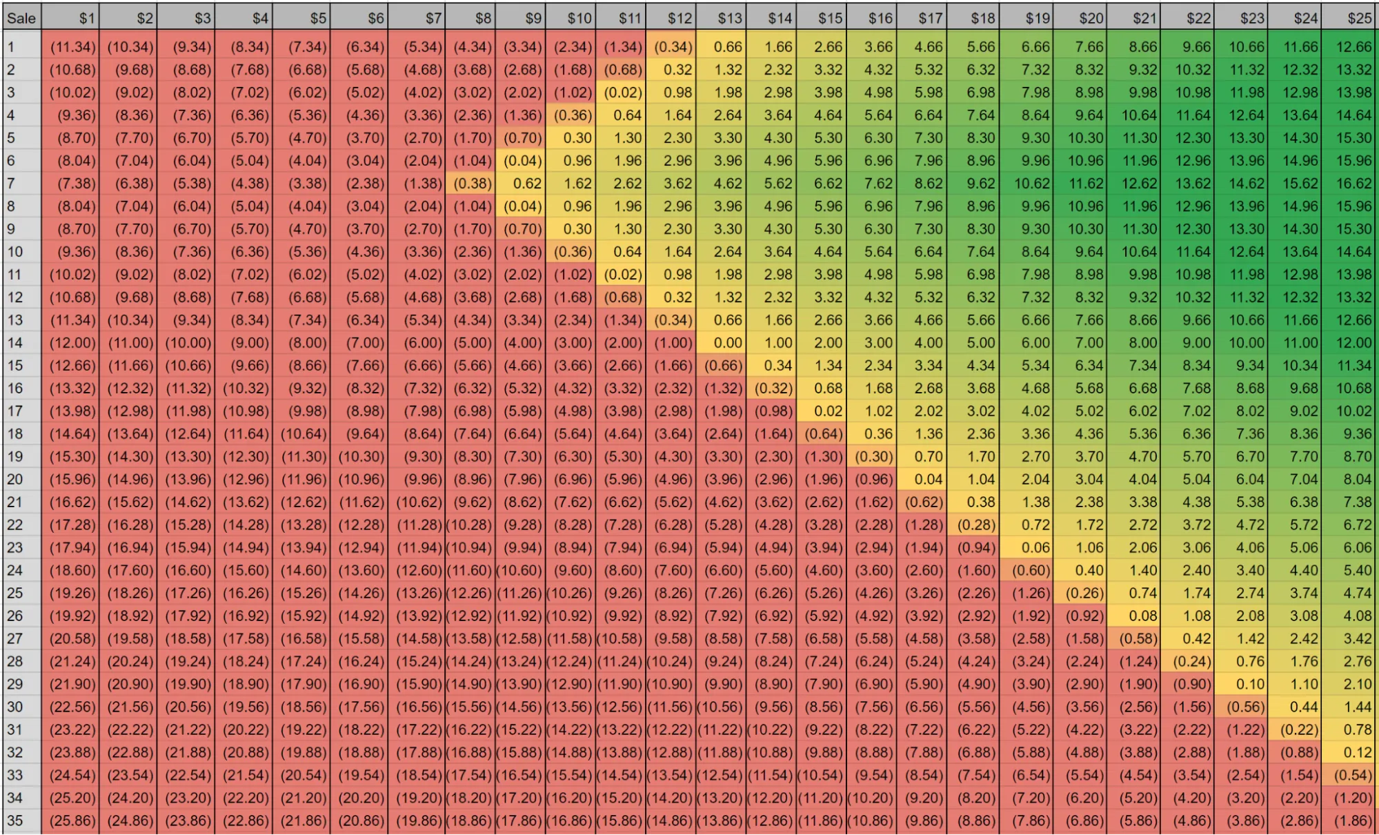
- Figure [Table 7.1]
Appendix II
Code
Full code for the simulation can be found at the links below.
Design
A high-level overview of the algorithms are:
- All AI-Firms are invited to set their price point
- In the Cournot Model, additionally set their Quantity Point
- For each consumer, if the consumer has more than $0, recursively take the following actions:
- Find the lowest priced AI-Firm
- If there are more than one AI-Firms offering, select one randomly from the set of lowest-price-vendors
- In the Cournot Model, check that the AI-Firms is willing to supply at least one additional product
- Purchase exactly one product from the AI-Firms
- Reduce consumer’s funds by the AI-Firm’s Vending Price
- Adjust the AI-Firm’s Marginal Transaction Cost, according to their marginal cost schedule -Adjust the vendor’s Current Account using the following equation where A is the vendor’s current account value, P is the vendor’s offered price, WP is the wholesale price faced by the vendor, MC is the vendor’s current Marginal Cost
- Find the lowest priced AI-Firm

- Exit the routine, returning the Current Account to the AI as its reward
Technical Limitation
The PPO algorithm used to conduct the research can settle into a non-optimal equilibrium if the simulator doesn’t sufficiently incentivise exploratory behaviour. Additionally, to save computation effort, the implementation shares an output space, meaning agents share the reward structure, which may incentivise an all boats rise with the tide type behaviour. Although this reflects the price-optimisation firm scenario outlined in The Economist’s article, where prices and rewards are known by all AI agents and distributed across many firms, it’s not generalisable across an entire economy, where AI-Firms are unlikely to share the same price-optimisation supplier.
Appendix III
| Table 1: Monopoly Quantitative Results - 2,000,000 training episodes | ||
|---|---|---|
| Model | Variable | Result |
| Bertrand | Avg Offered Price | $19 |
| Cournot | Avg Offered Price | $19 |
| Bertrand | Count Made Sale | 1 |
| Cournot | Count Made Sale | 1 |
| Bertrand | Average Final Vending Cost (MC) | $12.26 |
| Cournot | Average Final Vending Cost (MC) | $10.94 |
| Bertrand | Average Offered (no control mechanism) | N/A |
| Cournot | Average Offered | 23 |
| Bertrand | Total Sales | 25 |
| Cournot | Total Sales | 23 |
| Bertrand | Total Sales $ Value | 475 |
| Cournot | Total Sales $ Value | 437 |
| Table 2: Duopoly Quantitative Results - 3,000,000 training episodes | ||
|---|---|---|
| Model | Variable | Result |
| Bertrand | Avg Offered Price | $19 |
| Cournot | Avg Offered Price | $19 |
| Bertrand | Count Made Sale | 2 |
| Cournot | Count Made Sale | 2 |
| Bertrand | Average Final Vending Cost (MC) | $4.01 |
| Cournot | Average Final Vending Cost (MC) | $4.01 |
| Bertrand | Average Offered (no control mechanism) | N/A |
| Cournot | Average Offered | 25 |
| Bertrand | Total Sales | 25 |
| Cournot | Total Sales | 25 |
| Bertrand | Total Sales $ Value | 475 |
| Cournot | Total Sales $ Value | 475 |
| Table 3: Oligopoly Quantitative Results - 5,000,000 training episodes | ||
|---|---|---|
| Model | Variable | Result |
| Bertrand | Avg Offered Price | $18 |
| Cournot | Avg Offered Price | $19 |
| Bertrand | Count Made Sale | 3 |
| Cournot | Count Made Sale | 3-5 (fluctuating) |
| Bertrand | Average Final Vending Cost (MC) | $2.03 |
| Cournot | Average Final Vending Cost (MC) | $1.82 |
| Bertrand | Average Offered (no control mechanism) | N/A |
| Cournot | Average Offered | 19.65 |
| Bertrand | Total Sales | 25 |
| Cournot | Total Sales | 25 |
| Bertrand | Total Sales $ Value | 450 |
| Cournot | Total Sales $ Value | 475 |
| Table 4: Perfect Competition Quantitative Results - 15,000,000 training episodes | ||
|---|---|---|
| Model | Variable | Result |
| Bertrand | Avg Offered Price | $15 |
| Cournot | Avg Offered Price | $19 |
| Bertrand | Count Made Sale | 3 |
| Cournot | Count Made Sale | 2 |
| Bertrand | Average Final Vending Cost (MC) | $1.79 |
| Cournot | Average Final Vending Cost (MC) | $3.9 |
| Bertrand | Average Offered (no control mechanism) | N/A |
| Cournot | Average Offered | 12.80 |
| Bertrand | Total Sales | 25 |
| Cournot | Total Sales | 25 |
| Bertrand | Total Sales $ Value | 375 |
| Cournot | Total Sales $ Value | 475 |